The Xunta offers freely data regarding the locations and characteristics of the wind turbines in Galicia. For what concerns this post, I will just use this data to create visualizations of the turbines themselves.

The data

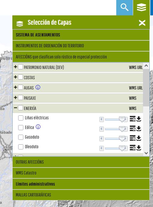
To download the data you should follow the link shown in the image, but basically to the layers button > Afeccións > Enerxía > Eólica.

This downloads a `.zip` file containing multiple formats, which is useful depending on your specific goal. For the visualizations in this article, I used the `.shp` (Shapefile) format, though the other files may contain different/more detailed data. In particular, the `.shp` has the following columns: 'OBJECTID', 'INFRAEST', 'NOME', 'ETRS89_X', 'ETRS89_Y', 'DIAM', 'ALT', 'NUM_ESTADO', 'SITUACION', 'geometry'. An example would be:

OBJECTID 2
INFRAEST AEROXERADOR
NOME PAXAREIRAS I
ETRS89_X 494628
ETRS89_Y 4.74572e+06
DIAM 44
ALT 40
NUM_ESTADO 5
SITUACION FUNCIONANDO, AUTORIZADO, EN OBRAS
geometry POINT (494628.4946999181 4745723.399695537)

As you can see and probably guess seeing the data, the `SITUACION` field is useless, every one has the same values. The rest of the data can be useful, though.

The visualization

Since the goal was just visualization, I wanted to try [kepler.gl](https://kepler.gl/). For the data to be correctly rendered there, it must be reprojected. The Xunta data is provided in CRS 29N (the UTM zone for Galicia), but Kepler requires WGS 84 (EPSG:4326), which is the global standard. Since millimetric precision is not a concern for these visuals, we can perform the conversion easily using geopandas

import geopandas as gpd

eolicos_gdf = gpd.read_file("your_path.shp")
eolicos_wgs84 = eolicos_gdf.to_crs("EPSG:4326")
eolicos_wgs84.to_file("your_output_file.geojson", driver="GeoJSON")

Additionally, for a more interesting visualization, i wanted to leverage the data within the .shp. This way, by reading both the height (ALT) and diameter (DIAM) we can create a more informative 3D visualization. For that, in terms of changes in the output file, we just need to extract the radious from the diameter and add it to the output .geojson. To do that we change the geometry from single points to actual polygons (circles):

import geopandas as gpd

eolicos_gdf = gpd.read_file("your_path.shp")
eolicos_gdf['geometry'] = eolicos_gdf.geometry.buffer(radii)
eolicos_wgs84 = eolicos_gdf.to_crs("EPSG:4326")
eolicos_wgs84.to_file("your_output_file.geojson", driver="GeoJSON")

Next, we can upload the file to kepler.gl and select the height field, mapping it to the ALT field in the geojson. That should output something like:

Additionally, using the plain .geojson I also created other visualization a heatmap-like one, to visualize where there are more wind turbines (the streght of the color is determined by height as a proxy for output power).

A “batea” is a kind of raft/floating structure made up of a lattice of wood beams combined with floats from which ropes, perpendicular to the raft iself, sink into the water allowing seafood, mostly mussels to grow.

Detecting these in visible Earth Observation (EO) images is relatively simple (given appropriate resolution) except for the fact that Galicia is notably cloudy. Thus, trying to monitor these with, for instance Sentinel 2, would mean staring the whole winter at a white wall of clouds. To build an observation system that works year-round, you have to drop the camera and pick up a microwave (only partially metaphorically). The tool for the job would be a Synthetic Aperture Radar (SAR) much like the one on Sentinel 1. Radar doesn’t care about clouds, in fact it goes through them. _What it does care about, a lot, is geometry.

Under normal circumstances, with calm water, a phenomenon called Specular reflection comes into play. SAR instruments cast microwaves from orbit to earth and then try to pick back what the terrain reflected. The smooth ocean surface deflects the radar pulse away from the satellite, causing calm water to appear dark. This easily contrasts with the bateas which are, essentially in this setting, corner reflectors. The pulse hits the flat water next to the raft, bounces upward into the vertical side of a beam and then shoots straight back at the satellite. This double bounce creates a strong signal that, despite the size of the bateas themselves and the low resolution of Sentinel 1, should be easily visible in the images.

The data

    def normalize_band(data, vmin, vmax):
        clipped = np.clip(data, vmin, vmax)
        return ((clipped - vmin) / (vmax - vmin) * 255.0).astype(np.uint8)

    vv_db = 10 * np.log10(vv_raw)
    vh_db = 10 * np.log10(vh_raw)
    diff_db = vv_db - vh_db

    R_channel = normalize_band(vv_db, -25, 0)
    G_channel = normalize_band(vh_db, -30, -5)
    B_channel = normalize_band(diff_db, 0, 15)

The output

Upon visualizing the images it became clear the bateas were visible despite their size (notice the little dots on the black sea in the images below).

Calm sea fake-color composite RGB

Calm sea VV Polarization

Calm sea VH Polarization

Choppy sea fake-color composite RGB

VV Polarization

VH Polarization